Transient Climate Evolution (TraCE)
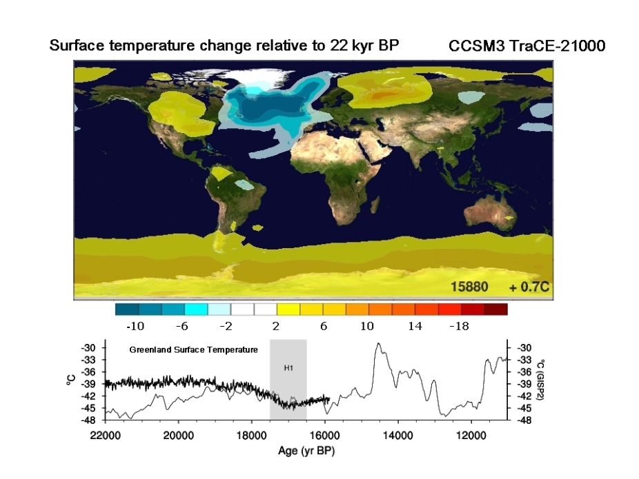
Transient evolution of surface temperature change simulated by CCSM3, click to view animation
The transient climate evolution of the last 21,000 years (Last Glacial Maximum to present) provides key observations for constraining climate sensitivity and understanding abrupt climate change. A synchronously coupled atmosphere-ocean general circulation model simulation of the last 21,000 years has been completed using the CCSM3. The transient simulation reproduces many major features of the deglacial climate evolution in Greenland, Antarctica, the tropical Pacific, and the Southern and Deep Oceans, thereby suggesting that CCSM3 exhibits reasonable climate sensistivity in those regions and is capable of simulating abrupt climate changes.
The TraCE-21000 project provides the four-dimensional model datasets to allow investigation of the coupled atmosphere-ocean-sea ice-land surface mechanisms and feedbacks that explain the evolution of the climate system over the last 21,000 years. It is also a resource for the paleodata research community providing a global framework for the synthesis of their data. Further, together the data and model results allow an assessment of the model capabilities. More information on the setup of this simulation can be found below as well as in the Ph.D dissertation of Dr. Feng He. Monthly time series of the atmospheric model variables are available for download on the Earth System Grid.
Model Description
The coupled atmosphere-ocean general circulation employed is the Community Climate System Model version 3 (CCSM3), centered at the National Center for Atmospheric Research (NCAR). CCSM3 is a global, coupled ocean-atmosphere-sea ice-land surface climate model without flux adjustment (Collins et al. 2006). All the simulations were performed at T31_gx3v5 resolution (Yeager et al., 2006; Otto-Bliesner et al., 2006) with a dynamic global vegetation model (DGVM).
The atmospheric model is the Community Atmospheric Model 3 (CAM3), a three-dimensional primitive equation model solved with the spectral method in the horizontal (T31, ~3.75o latitude-longitude resolution) and with 26 hybrid coordinate levels in the vertical.
The land model uses the same resolution as the atmosphere, and each grid box includes a hierarchy of land units, soil columns, and plant types. Glaciers, lakes, wetlands, urban areas, and vegetated regions can be specified in the land units. The dynamic vegetation parameterizations originated mostly from the Lund-Potsdam-Jena (LPJ)-DGVM, a model documented and evaluated against observations.
The ocean model is the NCAR implementation of the Parallel Ocean Program (POP) and is a three-dimensional primitive equation model in spherical polar coordinates with dipole grid and vertical z coordinate with 25 levels. The longitudinal resolution is 3.6o and the latitudinal resolution is variable, with finer resolution near the equator (~0.9o).
The sea ice model is the NCAR Community Sea Ice Model (CSIM), a dynamic-thermodynamic model that includes a subgrid-scale ice thickness distribution. The resolution of CSIM is identical to that of POP.
Forcings and boundary conditions
Orbital Forcing
According to Milankovitch theory, the ice age cycles are paced by the Earth's orbital variations, with Northern Hemisphere summer insolation intensity playing a dominant role in the growth and decay of Northern Hemisphere ice sheets. Orbital or astronomical forcing relates the well-known variations in the Earth's orbital parameters, eccentricity and precession, as well as changes in the axial tilt are well-known from precise astronomical calculations. These variations modulate the annual, seasonal, and latitudinal distributions and magnitudes of incoming solar radiation. The orbital parameters at LGM were only modestly different than today such that the latitudinal and seasonal distributions of incoming solar radiation were close to present. During the transition from LGM to present, the effects of precession (primarily) but also the axial tilt resulted in large and out-of-phase anomalies of Northern Hemisphere versus Southern Hemisphere summer insolation. These anomalies peaked at ~12-11 ka.
Atmospheric Greenhouse Gases (GHGs)
Ice cores indicate that atmospheric concentrations of carbon dioxide (CO2), methane (CH4), and nitrous oxide (N2O) have varied over glacial-interglacial cycles with systematically higher values during interglacials than during glacial periods. At the LGM, concentrations of these well-mixed GHGs were about 185 ppm for CO2, 350 ppb for CH4, and 200 ppb for N2O. In our simulation atmospheric CO2 started to rise at ~17 ka within Heinrich Stadial 1 (HS1) reaching 240 ppm by the onset of the Bolling-Allerod (BA) ~14.6 ka. After a ~5 ppm drop between the BA and Younger Dryas (YD), CO2 began rising again in the middle of the YD (~12.5 ka) and increased another 30 ppm from 235 to 265 ppm before the onset of the Holocene. The total CO2 rise during the last deglaciation was ~80 ppm (from 185 to 265 ppm). During the early Holocene, CO2 decreased by 5 ppm between 10 and 8 ka, and then rose again by 20 ppm to reach the pre-industrial level of 280 ppm. Atmospheric CH4 also started to rise at ~17 ka reaching ~650 ppb at the onset of the BA and then leveling off until the start of the YD. A sharp drop in CH4 occurred at the onset of the YD, usually attributed to a decreased wetlands production, followed by an abrupt increase at the end of the YD. During the Holocene, CH4 decreased until ~4 ka before resuming its increase to pre-industrial levels of 760 ppb. Atmospheric N2O had a similar transient evolution to atmospheric CH4, albeit with much smaller increases from 200 ppb at LGM to 270 ppb at pre-industrial.
Ice Sheets and Paleogeography
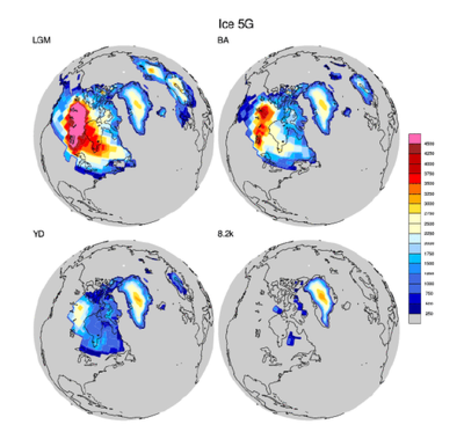
Massive ice sheets covered North America, Greenland and Eurasia at the LGM, with the height of the North American Ice Sheet being more than 4.5 km. In our simulation we adopt the ICE-5G (VM2) reconstruction of Peltier (2004). Between the LGM and BA, the Eurasian Ice Sheet retreated significantly with the areal coverage reduced by about two thirds. During this period, the areal coverage of the North American Ice Sheet remained more or less the same. However, the total volume of the North American Ice Sheet was reduced significantly. The North America Ice Sheets rapidly retreated between the Bolling-Allerod (BA) warm period and the cooler Younger Dryas (YD), during which time most of the Cordilleran Ice Sheet in western North America disappeared and the majority of the remaining Laurentide Ice Sheet was below 2 km. The Eurasian Ice Sheet eventually disappeared by ~8 ka, as did the Laurentide Ice Sheet by ~6 ka. The last deglaciation completely ended around 6 ka, when the mass balances of both the Greenland and Antarctic Ice Sheets reached their approximate Holocene equilibrium. As the ice sheets melted, sea level rose from the LGM low-stand of ~130m below present levels, flooding land that had been exposed at the low-stand. These geography changes are included in the simulation.
Watch the evolution of land ice represented by ICE-5G (VM2) (Peltier 2004) from 21ka to present day (animation courtesy of Jean-Yves Peterschmitt)
Meltwater Forcing
Meltwater fluxes from the retreating ice sheets started at 19ka, with meltwater from the Eurasian and Laurentide ice sheets added to the North Atlantic. The regions and intervals where the freshwater are added are based on our knowledge for geological records on which ice sheet was melting (see illustration). The flux of meltwater is also constrained by information on the rate of sea level rise during the last 21,000 years. In CCSM3 the meltwater discharge is added to the ocean model as a freshwater flux on the surface of the ocean. Meltwater discharge is usually expressed in units of m/kyr (meters of equivalent sea-level volume per thousand years) or Sv (1 Sv = 106 m3 s-1). Since the area of the ocean is about 3.61x10¹⁴ m2, 1 m of sea level rise per thousand years (m/kyr) means 3.61x10¹⁴ m3 volume of meltwater in 103 years, which is 0.011 m3 s-1, or 0.011 Sv. More details on the meltwater scenario are available.